Example usage
Here we will demonstrate how to use the stepsel package for stepwise selection of variables in a regression model and how to prepare categorical data for such a model.
# Importing the packages
import stepsel
import numpy as np
import statsmodels.api as sm
Load the data
First we load the data and take a look at the first few rows. It is soccer data from Czech First League.
dt = stepsel.datasets.load_soccer_data()
print(dt.shape, dt.columns)
(518, 24) Index(['match_id', 'match_datetime', 'team', 'hga', 'team_opp', 'goals',
       'goals_opp', 'yellow', 'yellow_opp', 'red', 'red_opp', 'penalty',
       'penalty_opp', 'fouls', 'fouls_opp', 'attacks', 'attacks_opp',
       'dangerous_attacks', 'dangerous_attacks_opp', 'ref_interv',
       'ref_interv_opp', 'ref_interv_per_attack', 'ref_interv_per_attack_opp',
       'ref_interv_per_attack_diff'],
      dtype='object')
dt.head()
| match_id | match_datetime | team | hga | team_opp | goals | goals_opp | yellow | yellow_opp | red | ... | fouls_opp | attacks | attacks_opp | dangerous_attacks | dangerous_attacks_opp | ref_interv | ref_interv_opp | ref_interv_per_attack | ref_interv_per_attack_opp | ref_interv_per_attack_diff | |
|---|---|---|---|---|---|---|---|---|---|---|---|---|---|---|---|---|---|---|---|---|---|
| 0 | 1 | 2023-05-14 18:00:00 | Bohemians | H | Slovácko | 0.0 | 0.0 | 2 | 2 | 0 | ... | 12.0 | 117.0 | 142.0 | 71.0 | 88.0 | 20.0 | 18.0 | 0.140845 | 0.153846 | -0.013001 |
| 1 | 2 | 2023-05-14 15:00:00 | Jablonec | H | Baník Ostrava | 1.0 | 1.0 | 1 | 1 | 0 | ... | 11.0 | 90.0 | 116.0 | 74.0 | 58.0 | 14.0 | 22.0 | 0.120690 | 0.244444 | -0.123755 |
| 2 | 3 | 2023-05-14 15:00:00 | Teplice | H | Zlín | 2.0 | 1.0 | 4 | 4 | 0 | ... | 14.0 | 118.0 | 134.0 | 54.0 | 62.0 | 30.0 | 26.0 | 0.223881 | 0.220339 | 0.003542 |
| 3 | 4 | 2023-05-14 15:00:00 | Zbrojovka Brno | H | Pardubice | 0.0 | 2.0 | 1 | 2 | 0 | ... | 14.0 | 99.0 | 126.0 | 57.0 | 76.0 | 17.0 | 36.0 | 0.134921 | 0.363636 | -0.228716 |
| 4 | 5 | 2023-05-13 18:00:00 | Sparta Praha | H | Slavia Praha | 3.0 | 2.0 | 1 | 2 | 0 | ... | 15.0 | 87.0 | 145.0 | 47.0 | 94.0 | 15.0 | 29.0 | 0.103448 | 0.333333 | -0.229885 |
5 rows × 24 columns
Binning the data
There are two ways to bin data in stepsel package: by specifying the cut points or optimal binning. We will demonstrate both.
By specifying the cut points
dt["fouls_opp_cat1"] = stepsel.binning.bin_values(dt["fouls_opp"], [8, 12, 16, 20])
dt["fouls_opp_cat1"].value_counts()
fouls_opp_cat1
(8, 12]      195
(12, 16]     167
(-Inf, 8]     84
(16, 20]      58
(20, Inf)     14
Name: count, dtype: int64
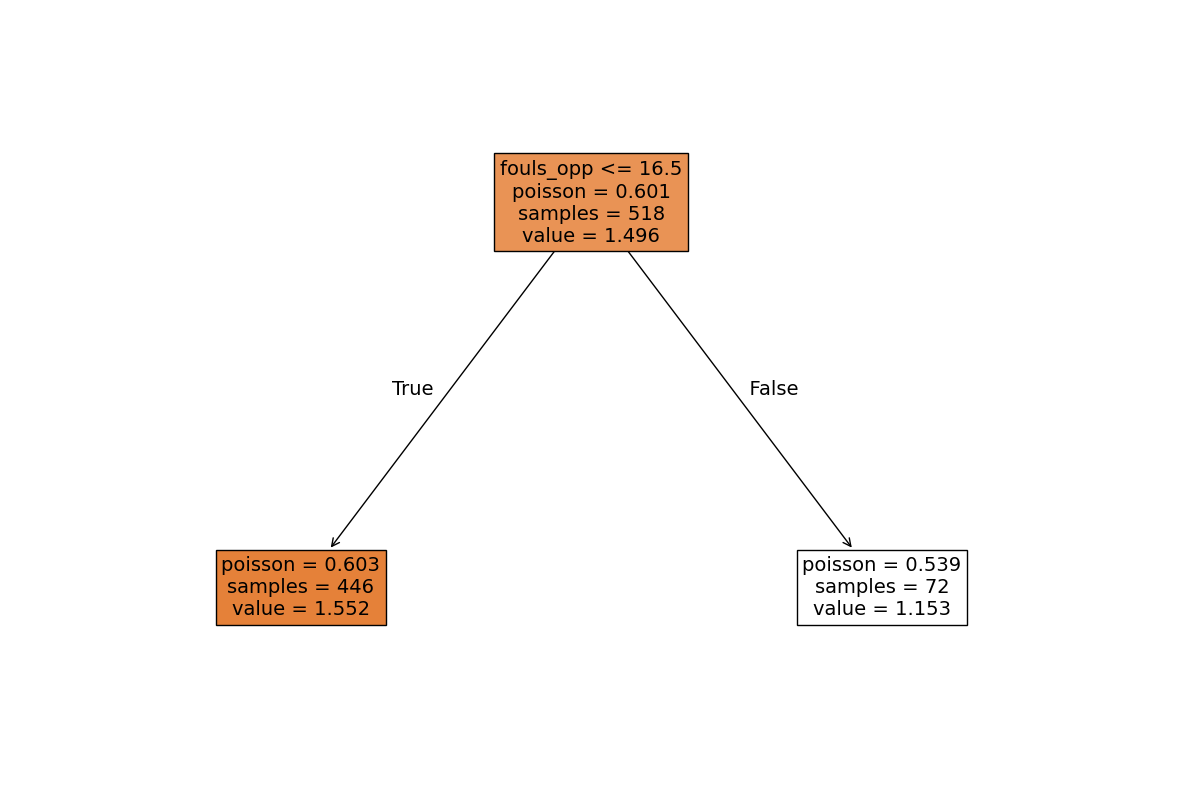
Optimal binning
Optimal binning can be time consuming, so when the data is large, and there are many cp values, they are grouped using K-means clustering and only the best clusters are used. This process is controlled by the Flow Parameters (see the docstring).
Other parameters are used to control the scikit-learn’s DecisionTreeRegressor, KMeans and GridSearchCV.
X = np.array(dt.loc[:, ["fouls_opp"]])
y = np.array(dt.loc[:, "goals"])

clf = stepsel.binning.optimal.OptimalBinningUsingDecisionTreeRegressor(
    criterion = 'poisson',
    scoring = "neg_mean_poisson_deviance",
    refit = "neg_mean_poisson_deviance",
    max_depth = 3
)
clf.fit(X, y) # Fit the model
clf.set_feature_names(["fouls_opp"]) # Set the feature names for the plot
clf.plot_tree((15,10)) # Plot the tree
Starting cross-validation for 58 cp values at 20:55:12.
Estimated runtime: 0.013480726877848308 minutes.
# Predicting the values
dt["fouls_opp_cat2"] = clf.predict(X)
dt["fouls_opp_cat2"].value_counts()
fouls_opp_cat2
1.551570    446
1.152778     72
Name: count, dtype: int64
# Creating the bins
dt["fouls_opp_cat2"] = clf.bin_values(dt["fouls_opp"])
dt["fouls_opp_cat2"] = dt["fouls_opp_cat2"].astype("category")
# Function to get the cut points can be used for any scikit-learn tree based model
# The final tree can be obtained from the cv_fit attribute of the model Log object
stepsel.binning.helper.get_tree_cut_points(clf.Log.fit_log["cv_fit"].best_estimator_, feature_names=["fouls_opp"])
{'fouls_opp': array([16.5])}
Setting the reference category
You can order any number of teams, the first one will be the reference category
dt["hga"] = stepsel.modeling.prep.relevel_categorical_variable(dt["hga"], ["H"])
dt["team"] = stepsel.modeling.prep.relevel_categorical_variable(dt["team"], ["Bohemians", "Jablonec"])
dt["team_opp"] = stepsel.modeling.prep.relevel_categorical_variable(dt["team_opp"], ["Bohemians", "Jablonec", "Teplice"])
dt["fouls_opp_cat1"] = stepsel.modeling.prep.relevel_categorical_variable(dt["fouls_opp_cat1"], ["(-Inf, 8]"])
Series is not categorical, converting to categorical.
Series is not categorical, converting to categorical.
Series is not categorical, converting to categorical.
Series is not categorical, converting to categorical.
Stepwise selection
The most important parameters for the selection are formula, include, slentry and slstay. Specifying the formula in R-style format, the variables to always include in the model, and the significance levels of the likelihood ratio test for entering and staying in the model.
# Parameters for the model
formula = "goals ~ team + hga + red_opp + fouls_opp_cat1 + fouls_opp_cat2"
include = ['ref_interv_per_attack * ref_interv_per_attack_opp', "penalty"]
slentry = 0.05
slstay = 0.10
family = sm.families.Poisson()
# Fitting the model
model1 = stepsel.modeling.stepwise_glm.StepwiseGLM(
    formula = formula,
    data = dt,
    include = include,
    slentry = slentry,
    slstay = slstay,
    family = family
)
model1.fit()
Best entry candidates:
          feature   p_value
0            team  0.000002
1             hga  0.000609
2         red_opp  0.005159
3  fouls_opp_cat2  0.013067
4  fouls_opp_cat1  0.060894
>> team entered the model.

Best removal candidates:
  feature   p_value
0    team  0.000002
>> No feature removed from the model.

Best entry candidates:
          feature   p_value
0             hga  0.000608
1         red_opp  0.004282
2  fouls_opp_cat2  0.045388
3  fouls_opp_cat1  0.160092
>> hga entered the model.

Best removal candidates:
  feature   p_value
0     hga  0.000608
1    team  0.000002
>> No feature removed from the model.

Best entry candidates:
          feature   p_value
0         red_opp  0.003997
1  fouls_opp_cat2  0.022037
2  fouls_opp_cat1  0.052854
>> red_opp entered the model.

Best removal candidates:
   feature   p_value
0  red_opp  0.003997
1      hga  0.000569
2     team  0.000002
>> No feature removed from the model.

Best entry candidates:
          feature   p_value
0  fouls_opp_cat2  0.037692
1  fouls_opp_cat1  0.108477
>> fouls_opp_cat2 entered the model.
Best removal candidates:
          feature   p_value
0  fouls_opp_cat2  0.037692
1         red_opp  0.006665
2             hga  0.000305
3            team  0.000004
>> No feature removed from the model.

Best entry candidates:
          feature   p_value
0  fouls_opp_cat1  0.353892
>> No feature entered the model.

Best removal candidates:
          feature   p_value
0  fouls_opp_cat2  0.037692
1         red_opp  0.006665
2             hga  0.000305
3            team  0.000004
>> No feature removed from the model.


Selection stopped because all candidates for removal are significant at the 0.1 level and no candidate for entry is significant at the 0.05 level.

                 Generalized Linear Model Regression Results
==============================================================================
Dep. Variable:                  goals   No. Observations:                  518
Model:                            GLM   Df Residuals:                      497
Model Family:                 Poisson   Df Model:                           20
Link Function:                    Log   Scale:                          1.0000
Method:                          IRLS   Log-Likelihood:                -754.52
Date:                Tue, 03 Sep 2024   Deviance:                       521.53
Time:                        20:55:13   Pearson chi2:                     442.
No. Iterations:                     5   Pseudo R-squ. (CS):             0.1771
Covariance Type:            nonrobust
=====================================================================================================================
                                                        coef    std err          z      P>|z|      [0.025      0.975]
---------------------------------------------------------------------------------------------------------------------
Intercept                                             0.6056      0.148      4.103      0.000       0.316       0.895
red_opp                                               0.3259      0.116      2.814      0.005       0.099       0.553
penalty                                               0.3239      0.084      3.867      0.000       0.160       0.488
team: Jablonec                                       -0.0641      0.199     -0.323      0.747      -0.453       0.325
team: Mladá Boleslav                                 -0.3061      0.211     -1.453      0.146      -0.719       0.107
team: Slavia Praha                                    0.5141      0.172      2.992      0.003       0.177       0.851
team: Baník Ostrava                                  -0.0717      0.199     -0.360      0.719      -0.462       0.318
team: Slovácko                                       -0.2592      0.210     -1.235      0.217      -0.670       0.152
team: Pardubice                                      -0.4425      0.226     -1.955      0.051      -0.886       0.001
team: Sparta Praha                                    0.2930      0.179      1.639      0.101      -0.057       0.643
team: Teplice                                        -0.3210      0.208     -1.545      0.122      -0.728       0.086
team: Sigma Olomouc                                  -0.0832      0.197     -0.423      0.672      -0.469       0.302
team: Zlín                                           -0.2405      0.211     -1.141      0.254      -0.654       0.173
team: Zbrojovka Brno                                 -0.2573      0.209     -1.231      0.218      -0.667       0.152
team: Hradec Králové                                 -0.2959      0.216     -1.367      0.172      -0.720       0.128
team: Slovan Liberec                                 -0.1045      0.203     -0.515      0.607      -0.502       0.293
team: České Budějovice                               -0.2703      0.213     -1.269      0.204      -0.688       0.147
team: Viktoria Plzeň                                  0.0649      0.189      0.343      0.732      -0.306       0.436
hga: A                                               -0.2616      0.073     -3.597      0.000      -0.404      -0.119
fouls_opp_cat2: (16.5, Inf)                          -0.2456      0.121     -2.024      0.043      -0.483      -0.008
ref_interv_per_attack * ref_interv_per_attack_opp    -1.5845      1.311     -1.208      0.227      -4.154       0.985
=====================================================================================================================
<stepsel.modeling.stepwise_glm.StepwiseGLM at 0x7f33444bee40>
Refitting the model
After the selection it is possible to specify different model formula and use the Log of the previously fitted model to speed up the selection. This is useful when the data is large and the selection is time consuming. The same partial models during the selection won’t be fitted again. Only use this functionality when the data has not changed!
# The new formula including the team_opp variable
formula_new = "goals ~ team + hga + red_opp + fouls_opp_cat1 + fouls_opp_cat2 + team_opp"
model2 = stepsel.modeling.stepwise_glm.StepwiseGLM(
    formula = formula_new,
    data = dt,
    include = include,
    slentry = slentry,
    slstay = slstay,
    model_fit_log = model1.model_fit_log, # Use the previous model fit Log object
    family = sm.families.Poisson()
)
model2.fit()
Best entry candidates:
          feature   p_value
0            team  0.000002
1        team_opp  0.000284
2             hga  0.000609
3         red_opp  0.005159
4  fouls_opp_cat2  0.013067
>> team entered the model.

Best removal candidates:
  feature   p_value
0    team  0.000002
>> No feature removed from the model.

Best entry candidates:
          feature   p_value
0        team_opp  0.000392
1             hga  0.000608
2         red_opp  0.004282
3  fouls_opp_cat2  0.045388
4  fouls_opp_cat1  0.160092
>> team_opp entered the model.

Best removal candidates:
    feature   p_value
0  team_opp  0.000392
1      team  0.000003
>> No feature removed from the model.

Best entry candidates:
          feature   p_value
0             hga  0.000621
1         red_opp  0.005264
2  fouls_opp_cat2  0.078540
3  fouls_opp_cat1  0.131029
>> hga entered the model.
Best removal candidates:
    feature   p_value
0       hga  0.000621
1  team_opp  0.000397
2      team  0.000003
>> No feature removed from the model.

Best entry candidates:
          feature   p_value
0         red_opp  0.005355
1  fouls_opp_cat1  0.044937
2  fouls_opp_cat2  0.049454
>> red_opp entered the model.

Best removal candidates:
    feature   p_value
0   red_opp  0.005355
1       hga  0.000632
2  team_opp  0.000478
3      team  0.000003
>> No feature removed from the model.
Best entry candidates:
          feature   p_value
0  fouls_opp_cat2  0.096376
1  fouls_opp_cat1  0.097127
>> No feature entered the model.

Best removal candidates:
    feature   p_value
0   red_opp  0.005355
1       hga  0.000632
2  team_opp  0.000478
3      team  0.000003
>> No feature removed from the model.


Selection stopped because all candidates for removal are significant at the 0.1 level and no candidate for entry is significant at the 0.05 level.

                 Generalized Linear Model Regression Results
==============================================================================
Dep. Variable:                  goals   No. Observations:                  518
Model:                            GLM   Df Residuals:                      483
Model Family:                 Poisson   Df Model:                           34
Link Function:                    Log   Scale:                          1.0000
Method:                          IRLS   Log-Likelihood:                -736.76
Date:                Tue, 03 Sep 2024   Deviance:                       486.00
Time:                        20:55:13   Pearson chi2:                     405.
No. Iterations:                     5   Pseudo R-squ. (CS):             0.2316
Covariance Type:            nonrobust
=====================================================================================================================
                                                        coef    std err          z      P>|z|      [0.025      0.975]
---------------------------------------------------------------------------------------------------------------------
Intercept                                             0.6859      0.204      3.367      0.001       0.287       1.085
red_opp                                               0.3446      0.120      2.880      0.004       0.110       0.579
penalty                                               0.3079      0.085      3.633      0.000       0.142       0.474
team: Jablonec                                       -0.1051      0.200     -0.526      0.599      -0.496       0.286
team: Mladá Boleslav                                 -0.3335      0.212     -1.576      0.115      -0.748       0.081
team: Slavia Praha                                    0.4651      0.173      2.691      0.007       0.126       0.804
team: Baník Ostrava                                  -0.1165      0.200     -0.584      0.559      -0.508       0.275
team: Slovácko                                       -0.3340      0.211     -1.585      0.113      -0.747       0.079
team: Pardubice                                      -0.4832      0.227     -2.129      0.033      -0.928      -0.038
team: Sparta Praha                                    0.2698      0.180      1.501      0.133      -0.082       0.622
team: Teplice                                        -0.3210      0.208     -1.541      0.123      -0.729       0.087
team: Sigma Olomouc                                  -0.1164      0.197     -0.590      0.556      -0.503       0.271
team: Zlín                                           -0.2897      0.212     -1.369      0.171      -0.704       0.125
team: Zbrojovka Brno                                 -0.2716      0.210     -1.294      0.196      -0.683       0.140
team: Hradec Králové                                 -0.3747      0.217     -1.727      0.084      -0.800       0.051
team: Slovan Liberec                                 -0.1739      0.204     -0.853      0.393      -0.573       0.226
team: České Budějovice                               -0.2836      0.214     -1.326      0.185      -0.703       0.136
team: Viktoria Plzeň                                  0.0574      0.190      0.302      0.763      -0.315       0.430
hga: A                                               -0.2470      0.073     -3.404      0.001      -0.389      -0.105
team_opp: Jablonec                                    0.1064      0.187      0.570      0.569      -0.260       0.472
team_opp: Teplice                                     0.1953      0.184      1.064      0.287      -0.165       0.555
team_opp: Mladá Boleslav                             -0.1597      0.202     -0.791      0.429      -0.556       0.236
team_opp: Slavia Praha                               -0.6235      0.229     -2.718      0.007      -1.073      -0.174
team_opp: Baník Ostrava                              -0.1468      0.204     -0.720      0.471      -0.546       0.253
team_opp: Slovácko                                   -0.2684      0.205     -1.310      0.190      -0.670       0.133
team_opp: Pardubice                                   0.0812      0.188      0.432      0.666      -0.287       0.449
team_opp: Sparta Praha                               -0.4883      0.223     -2.192      0.028      -0.925      -0.052
team_opp: Sigma Olomouc                              -0.1868      0.202     -0.925      0.355      -0.583       0.209
team_opp: Zlín                                        0.1161      0.188      0.619      0.536      -0.252       0.484
team_opp: Zbrojovka Brno                              0.1574      0.185      0.849      0.396      -0.206       0.521
team_opp: Hradec Králové                             -0.3510      0.208     -1.685      0.092      -0.759       0.057
team_opp: Slovan Liberec                             -0.1634      0.199     -0.820      0.412      -0.554       0.227
team_opp: České Budějovice                            0.0914      0.188      0.485      0.627      -0.278       0.461
team_opp: Viktoria Plzeň                             -0.3707      0.214     -1.732      0.083      -0.790       0.049
ref_interv_per_attack * ref_interv_per_attack_opp    -1.1145      1.309     -0.852      0.394      -3.679       1.450
=====================================================================================================================
<stepsel.modeling.stepwise_glm.StepwiseGLM at 0x7f3342816870>
# Print the summary of the final model. The extracted model is statsmodels object.
final_model = model2.current_model
print(final_model.summary())
                 Generalized Linear Model Regression Results
==============================================================================
Dep. Variable:                  goals   No. Observations:                  518
Model:                            GLM   Df Residuals:                      483
Model Family:                 Poisson   Df Model:                           34
Link Function:                    Log   Scale:                          1.0000
Method:                          IRLS   Log-Likelihood:                -736.76
Date:                Tue, 03 Sep 2024   Deviance:                       486.00
Time:                        20:55:14   Pearson chi2:                     405.
No. Iterations:                     5   Pseudo R-squ. (CS):             0.2316
Covariance Type:            nonrobust
=====================================================================================================================
                                                        coef    std err          z      P>|z|      [0.025      0.975]
---------------------------------------------------------------------------------------------------------------------
Intercept                                             0.6859      0.204      3.367      0.001       0.287       1.085
red_opp                                               0.3446      0.120      2.880      0.004       0.110       0.579
penalty                                               0.3079      0.085      3.633      0.000       0.142       0.474
team: Jablonec                                       -0.1051      0.200     -0.526      0.599      -0.496       0.286
team: Mladá Boleslav                                 -0.3335      0.212     -1.576      0.115      -0.748       0.081
team: Slavia Praha                                    0.4651      0.173      2.691      0.007       0.126       0.804
team: Baník Ostrava                                  -0.1165      0.200     -0.584      0.559      -0.508       0.275
team: Slovácko                                       -0.3340      0.211     -1.585      0.113      -0.747       0.079
team: Pardubice                                      -0.4832      0.227     -2.129      0.033      -0.928      -0.038
team: Sparta Praha                                    0.2698      0.180      1.501      0.133      -0.082       0.622
team: Teplice                                        -0.3210      0.208     -1.541      0.123      -0.729       0.087
team: Sigma Olomouc                                  -0.1164      0.197     -0.590      0.556      -0.503       0.271
team: Zlín                                           -0.2897      0.212     -1.369      0.171      -0.704       0.125
team: Zbrojovka Brno                                 -0.2716      0.210     -1.294      0.196      -0.683       0.140
team: Hradec Králové                                 -0.3747      0.217     -1.727      0.084      -0.800       0.051
team: Slovan Liberec                                 -0.1739      0.204     -0.853      0.393      -0.573       0.226
team: České Budějovice                               -0.2836      0.214     -1.326      0.185      -0.703       0.136
team: Viktoria Plzeň                                  0.0574      0.190      0.302      0.763      -0.315       0.430
hga: A                                               -0.2470      0.073     -3.404      0.001      -0.389      -0.105
team_opp: Jablonec                                    0.1064      0.187      0.570      0.569      -0.260       0.472
team_opp: Teplice                                     0.1953      0.184      1.064      0.287      -0.165       0.555
team_opp: Mladá Boleslav                             -0.1597      0.202     -0.791      0.429      -0.556       0.236
team_opp: Slavia Praha                               -0.6235      0.229     -2.718      0.007      -1.073      -0.174
team_opp: Baník Ostrava                              -0.1468      0.204     -0.720      0.471      -0.546       0.253
team_opp: Slovácko                                   -0.2684      0.205     -1.310      0.190      -0.670       0.133
team_opp: Pardubice                                   0.0812      0.188      0.432      0.666      -0.287       0.449
team_opp: Sparta Praha                               -0.4883      0.223     -2.192      0.028      -0.925      -0.052
team_opp: Sigma Olomouc                              -0.1868      0.202     -0.925      0.355      -0.583       0.209
team_opp: Zlín                                        0.1161      0.188      0.619      0.536      -0.252       0.484
team_opp: Zbrojovka Brno                              0.1574      0.185      0.849      0.396      -0.206       0.521
team_opp: Hradec Králové                             -0.3510      0.208     -1.685      0.092      -0.759       0.057
team_opp: Slovan Liberec                             -0.1634      0.199     -0.820      0.412      -0.554       0.227
team_opp: České Budějovice                            0.0914      0.188      0.485      0.627      -0.278       0.461
team_opp: Viktoria Plzeň                             -0.3707      0.214     -1.732      0.083      -0.790       0.049
ref_interv_per_attack * ref_interv_per_attack_opp    -1.1145      1.309     -0.852      0.394      -3.679       1.450
=====================================================================================================================
Prepering model matrix for other models
The stepsel package can be used to prepare the model matrix for other models. The prepare_model_matrix function is used for this purpose using the convienient formula syntax.
Interaction terms of two variables are supported.
# Prepare the model matrix
formula = "goals ~ team + hga * penalty"
y, X, feature_ids = stepsel.modeling.prep.prepare_model_matrix(formula, dt)
Fit statsmodels model with prepared model matrix using stepsel
# Train-test split based on the match_id
train_filter = dt["match_id"] <= 200
y_train = y[train_filter]
X_train = X.loc[train_filter,:].copy()
y_test = y[~train_filter]
X_test = X.loc[~train_filter,:].copy()
# Fit the model
model3 = sm.GLM(endog = y_train,
              exog = X_train,
              family = family)
model3 = model3.fit()
print(model3.summary())
                 Generalized Linear Model Regression Results
==============================================================================
Dep. Variable:                  goals   No. Observations:                  400
Model:                            GLM   Df Residuals:                      382
Model Family:                 Poisson   Df Model:                           17
Link Function:                    Log   Scale:                          1.0000
Method:                          IRLS   Log-Likelihood:                -593.90
Date:                Tue, 03 Sep 2024   Deviance:                       423.76
Time:                        20:55:14   Pearson chi2:                     369.
No. Iterations:                     5   Pseudo R-squ. (CS):             0.1442
Covariance Type:            nonrobust
==========================================================================================
                             coef    std err          z      P>|z|      [0.025      0.975]
------------------------------------------------------------------------------------------
Intercept                  0.4030      0.159      2.531      0.011       0.091       0.715
team: Jablonec            -0.0476      0.226     -0.211      0.833      -0.490       0.394
team: Mladá Boleslav      -0.2761      0.244     -1.131      0.258      -0.755       0.202
team: Slavia Praha         0.4624      0.201      2.295      0.022       0.067       0.857
team: Baník Ostrava       -0.0086      0.224     -0.038      0.969      -0.448       0.431
team: Slovácko            -0.2853      0.244     -1.171      0.242      -0.763       0.192
team: Pardubice           -0.3462      0.249     -1.390      0.165      -0.834       0.142
team: Sparta Praha         0.4073      0.201      2.031      0.042       0.014       0.800
team: Teplice             -0.2247      0.234     -0.960      0.337      -0.683       0.234
team: Sigma Olomouc        0.0312      0.221      0.141      0.888      -0.403       0.465
team: Zlín                -0.1886      0.239     -0.790      0.430      -0.657       0.279
team: Zbrojovka Brno      -0.3861      0.248     -1.557      0.120      -0.872       0.100
team: Hradec Králové      -0.2945      0.243     -1.210      0.226      -0.772       0.183
team: Slovan Liberec      -0.1769      0.235     -0.754      0.451      -0.637       0.283
team: České Budějovice    -0.2186      0.239     -0.915      0.360      -0.687       0.250
team: Viktoria Plzeň       0.1407      0.214      0.656      0.512      -0.279       0.561
hga: H * penalty           0.4112      0.120      3.426      0.001       0.176       0.646
hga: A * penalty           0.2397      0.112      2.131      0.033       0.019       0.460
==========================================================================================
Fixing some of the variables coefficients
It is possible to fix some of the variables coefficients to a specific value using offset. This is particularly useful when the variable is a factor and one or more of its levels are not well fitted by the model.
# Fix some of the coefficients - use the names of the coefficients from the summary
adjusted_coeffs = {"team: Baník Ostrava": 0.00,
                   "hga: H * penalty": 0.45
}
# Adjust the model matrix and offset
X_train, X_test, offset_train, offset_test = stepsel.modeling.prep.model_matrix.adjust_model_matrix([X_train, X_test], adjusted_coeffs)
# Fit the final model using the adjusted model matrix and offset
model_final2 = sm.GLM(endog = y_train,
              exog = X_train,
              family = family,
              offset = offset_train)
model_final2 = model_final2.fit()
print(model_final2.summary())
                 Generalized Linear Model Regression Results
==============================================================================
Dep. Variable:                  goals   No. Observations:                  400
Model:                            GLM   Df Residuals:                      384
Model Family:                 Poisson   Df Model:                           15
Link Function:                    Log   Scale:                          1.0000
Method:                          IRLS   Log-Likelihood:                -593.96
Date:                Tue, 03 Sep 2024   Deviance:                       423.87
Time:                        20:55:14   Pearson chi2:                     370.
No. Iterations:                     5   Pseudo R-squ. (CS):             0.1189
Covariance Type:            nonrobust
==========================================================================================
                             coef    std err          z      P>|z|      [0.025      0.975]
------------------------------------------------------------------------------------------
Intercept                  0.3918      0.112      3.492      0.000       0.172       0.612
team: Jablonec            -0.0413      0.197     -0.209      0.834      -0.428       0.345
team: Mladá Boleslav      -0.2652      0.217     -1.223      0.221      -0.690       0.160
team: Slavia Praha         0.4703      0.169      2.785      0.005       0.139       0.801
team: Slovácko            -0.2766      0.217     -1.276      0.202      -0.701       0.148
team: Pardubice           -0.3373      0.223     -1.514      0.130      -0.774       0.099
team: Sparta Praha         0.4092      0.169      2.426      0.015       0.079       0.740
team: Teplice             -0.2206      0.207     -1.065      0.287      -0.627       0.185
team: Sigma Olomouc        0.0376      0.192      0.196      0.845      -0.339       0.414
team: Zlín                -0.1821      0.212     -0.860      0.390      -0.597       0.233
team: Zbrojovka Brno      -0.3819      0.223     -1.716      0.086      -0.818       0.054
team: Hradec Králové      -0.2878      0.217     -1.327      0.185      -0.713       0.137
team: Slovan Liberec      -0.1685      0.207     -0.814      0.416      -0.574       0.237
team: České Budějovice    -0.2099      0.212     -0.992      0.321      -0.625       0.205
team: Viktoria Plzeň       0.1474      0.184      0.802      0.423      -0.213       0.508
hga: A * penalty           0.2439      0.112      2.184      0.029       0.025       0.463
==========================================================================================
Scoring the model
The model can be scored via standard statsmodels API. stepsel package provides a scoring_table object, which handles the fixed variables and the offset in a straightforward way. It is also possible to generate SQL code for scoring the model in the database.
# Create scoring table
# Notice the fixed coefficients are also used in the scoring table
# You can also create the scoring table from csv file or pandas DataFrame.
scoring_table = stepsel.modeling.predict.ScoringTableGLM.from_glm_model(model_final2, adjusted_coeffs)
print(scoring_table)
ScoringTableGLM(scoring_table=         var1     var2        level_var1 level_var2  estimate
0   Intercept     None              None       None  0.391757
1        team     None  České Budějovice       None -0.209868
2        team     None              Zlín       None -0.182095
3        team     None    Zbrojovka Brno       None -0.381924
4        team     None    Viktoria Plzeň       None  0.147379
5        team     None           Teplice       None -0.220638
6        team     None      Sparta Praha       None  0.409163
7        team     None          Slovácko       None -0.276560
8        team     None    Slovan Liberec       None -0.168498
9        team     None      Slavia Praha       None  0.470338
10       team     None     Sigma Olomouc       None  0.037562
11       team     None         Pardubice       None -0.337274
12       team     None    Mladá Boleslav       None -0.265193
13       team     None          Jablonec       None -0.041279
14       team     None    Hradec Králové       None -0.287798
15       team     None     Baník Ostrava       None  0.000000
16        hga  penalty                 H       None  0.450000
17        hga  penalty                 A       None  0.243900)
# For prediction, prepare the full model matrix
y, X_full, feature_ids_full = stepsel.modeling.prep.prepare_model_matrix(formula, dt, drop_first=False)

# There is a method to predict the linear predictor of the model, which can be used to calculate the predictions
dt["preds"] = np.exp(scoring_table.predict_linear(X_full))
# Generate the SQL code for the model (microsoft SQL Server flavor)
print(scoring_table.sql(format=True))
 + 0.39175660628921727
 + case  when TRIM(CAST(team as varchar(999))) = 'České Budějovice' then -0.209868356396289
 when TRIM(CAST(team as varchar(999))) = 'Zlín' then -0.18209532272001622
 when TRIM(CAST(team as varchar(999))) = 'Zbrojovka Brno' then -0.38192399630625423
 when TRIM(CAST(team as varchar(999))) = 'Viktoria Plzeň' then 0.14737941642116714
 when TRIM(CAST(team as varchar(999))) = 'Teplice' then -0.22063773340931692
 when TRIM(CAST(team as varchar(999))) = 'Sparta Praha' then 0.4091626261463444
 when TRIM(CAST(team as varchar(999))) = 'Slovácko' then -0.2765597308949606
 when TRIM(CAST(team as varchar(999))) = 'Slovan Liberec' then -0.16849805557501135
 when TRIM(CAST(team as varchar(999))) = 'Slavia Praha' then 0.4703384015175227
 when TRIM(CAST(team as varchar(999))) = 'Sigma Olomouc' then 0.037561752737359344
 when TRIM(CAST(team as varchar(999))) = 'Pardubice' then -0.3372735198024266
 when TRIM(CAST(team as varchar(999))) = 'Mladá Boleslav' then -0.2651933788212607
 when TRIM(CAST(team as varchar(999))) = 'Jablonec' then -0.041278776042565524
 when TRIM(CAST(team as varchar(999))) = 'Hradec Králové' then -0.28779833962517487
 when TRIM(CAST(team as varchar(999))) = 'Baník Ostrava' then 0.0 else 0.0 end
 + case  when TRIM(CAST(hga as varchar(999))) = 'H' then penalty * 0.45
 when TRIM(CAST(hga as varchar(999))) = 'A' then penalty * 0.24390049563090516 else 0.0 end
Verifying the model
For quick verification of the model, one can use the group_over_columns function, which goes over the specified columns and applies the specified grouping dictionary. This is built on top of the pandas groupby function.
# Evaluate the model. Note you can evaluate any combination of variables.
vars2eval = ["team", "hga", "penalty", "fouls_opp_cat2", ["hga", "penalty"]]
evaluation_train = stepsel.tools.group_over_columns(dt.loc[train_filter,], vars2eval, {"goals": "mean", "preds": "mean" })
evaluation_test = stepsel.tools.group_over_columns(dt.loc[~train_filter,:], vars2eval, {"goals": "mean", "preds": "mean"})
# One can see that rather simple descriptive model fits the data reasonably well, even though it was constructed only to demonstrate the package.
# The biggest discrepancy is in matches with penalty, and for the teams of Slavia Praha and Sparta Praha. This has its reasons,
# and Czech football fans will have their own opinions on that.
print(evaluation_train, evaluation_test, sep="\n\n")
        variable_1           level_1 variable_2  level_2     goals     preds
0             team         Bohemians        NaN      NaN  1.640000  1.636806
1             team          Jablonec        NaN      NaN  1.520000  1.520000
2             team    Mladá Boleslav        NaN      NaN  1.160000  1.160000
3             team      Slavia Praha        NaN      NaN  2.560000  2.560000
4             team     Baník Ostrava        NaN      NaN  1.560000  1.563194
5             team          Slovácko        NaN      NaN  1.160000  1.160000
6             team         Pardubice        NaN      NaN  1.080000  1.080000
7             team      Sparta Praha        NaN      NaN  2.560000  2.560000
8             team           Teplice        NaN      NaN  1.320000  1.320000
9             team     Sigma Olomouc        NaN      NaN  1.640000  1.640000
10            team              Zlín        NaN      NaN  1.291667  1.291667
11            team    Zbrojovka Brno        NaN      NaN  1.080000  1.080000
12            team    Hradec Králové        NaN      NaN  1.160000  1.160000
13            team    Slovan Liberec        NaN      NaN  1.320000  1.320000
14            team  České Budějovice        NaN      NaN  1.240000  1.240000
15            team    Viktoria Plzeň        NaN      NaN  1.807692  1.807692
16             hga                 H        NaN      NaN  1.755000  1.542806
17             hga                 A        NaN      NaN  1.260000  1.472194
18         penalty               0.0        NaN      NaN  1.380403  1.387885
19         penalty               1.0        NaN      NaN  2.361702  2.193053
20         penalty               2.0        NaN      NaN  2.166667  3.055077
21  fouls_opp_cat2      (-Inf, 16.5]        NaN      NaN  1.567251  1.512505
22  fouls_opp_cat2       (16.5, Inf)        NaN      NaN  1.155172  1.477987
23             hga                 H    penalty      0.0  1.641618  1.404335
24             hga                 H    penalty      1.0  2.600000  2.379531
25             hga                 H    penalty      2.0  1.000000  3.061540
26             hga                 A    penalty      0.0  1.120690  1.371529
27             hga                 A    penalty      1.0  2.090909  1.981147
28             hga                 A    penalty      2.0  2.750000  3.051845

        variable_1           level_1 variable_2  level_2     goals     preds
0             team         Bohemians        NaN      NaN  1.625000  1.635771
1             team          Jablonec        NaN      NaN  1.428571  1.535011
2             team    Mladá Boleslav        NaN      NaN  1.428571  1.363987
3             team      Slavia Praha        NaN      NaN  3.375000  2.449881
4             team     Baník Ostrava        NaN      NaN  1.285714  1.479578
5             team          Slovácko        NaN      NaN  1.375000  1.201807
6             team         Pardubice        NaN      NaN  0.571429  1.055995
7             team      Sparta Praha        NaN      NaN  1.500000  2.544079
8             team           Teplice        NaN      NaN  1.142857  1.282971
9             team     Sigma Olomouc        NaN      NaN  1.125000  1.645341
10            team              Zlín        NaN      NaN  1.000000  1.233260
11            team    Zbrojovka Brno        NaN      NaN  1.857143  1.049731
12            team    Hradec Králové        NaN      NaN  1.000000  1.109554
13            team    Slovan Liberec        NaN      NaN  1.714286  1.250144
14            team  České Budějovice        NaN      NaN  1.000000  1.199480
15            team    Viktoria Plzeň        NaN      NaN  1.714286  1.714525
16             hga                 H        NaN      NaN  1.440678  1.545113
17             hga                 A        NaN      NaN  1.474576  1.454344
18         penalty               0.0        NaN      NaN  1.428571  1.411392
19         penalty               1.0        NaN      NaN  1.692308  2.213212
20  fouls_opp_cat2      (-Inf, 16.5]        NaN      NaN  1.500000  1.513460
21  fouls_opp_cat2       (16.5, Inf)        NaN      NaN  1.142857  1.397720
22             hga                 H    penalty      0.0  1.440000  1.400752
23             hga                 H    penalty      1.0  1.444444  2.347115
24             hga                 A    penalty      0.0  1.418182  1.421065
25             hga                 A    penalty      1.0  2.250000  1.911932